Gravitational Waves

Quantum Physics
Relativity and Cosmology
Albert Einstein predicted the relativity of gravitational waves in early 1916 on the basis of general relativity, the existence of gravitational waves is still an active topic of research.
Ripples in space time that may provide clues about the origins of our universe, gravitational waves are extremely weak and difficult to detect. In general relativity, gravitation is explained through the curvature of spacetime. Massive objects bend spacetime, and the curvature of spacetime tells objects how to move. It is the influence of curved spacetime that we call gravity.

There is an ongoing effort to detect gravitational waves using interferometers on the ground and in space, and through accurate timing of pulsars. First detections are expected within the next few years and these observations have the potential to transform our understanding of astrophysics, cosmology and fundamental physics. Members of the IoA Gravity Group are involved with all aspects of this work on gravitational wave detection, including source modeling, data analysis and exploring the scientific exploitation of the data.

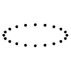
There is a global community of scientists and engineers currently working towards the first direct detection of gravitational waves. To visualize the effect of a gravitational wave passing imagine you have a ring of particles lying in a plane. When the wave passes through the ring it is stretched and squeezed, although the area enclosed remains the same. Detectors work by trying to measure the differences in length across a detector produced as a wave passes. The fractional changes in length are tiny, about one part in 1021, so the measurements are extremely difficult. That is the same as trying to measure the distance from the Earth to the Sun to the accuracy of the size of a hydrogen atom!

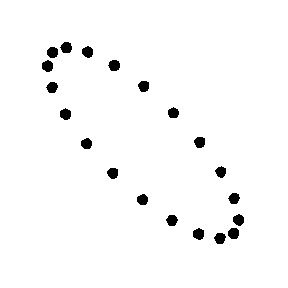The effects of the two gravitational wave polarizations, plus (+) and cross (×), on a ring of particles. The wave would be travelling out of the screen.

Dr. Mavalvala’s research is at the forefront of new detectors that are part of the Laser Interferometer Gravitational-Wave Observatory (LIGO), a major collaborative project operated by Caltech and MIT. Her work is revealing new insights about the role of quantum effects: the sensitivity of the upcoming generation of interferometric gravitational wave detectors is expected to be predominantly limited by quantum optical noise. Dr. Mavalvala will explore the origins of these quantum limits, and describe experimental progress toward circumventing them.

Just like electromagnetic radiation, gravitational radiation comes in a range of frequencies. The frequency is set by the scale of the system producing the radiation. Different parts of the spectrum can be observed using different detectors.

GWspec
The gravitational wave spectrum, sources and detectors. Credit: Harvard University

Astrophysics

Einstein’s equations form the fundamental law of general relativity. The curvature of spacetime can be expressed mathematically using the metric tensor — denoted $g_{\mu \nu} \,$ . The metric holds information regarding how distances are measured in the space under consideration. Because the propagation of gravitational waves through space and time change distances, we will need to use this to find the solution to the wave equation.

Spacetime curvature is also expressed with respect to a covariant derivative, $\nabla \,$ , in the form of the Einstein tensor, $G_{\mu \nu}$ . This curvature is related to the stress–energy tensor, $T_{\mu\nu}$ , by the key equation

G_{\mu \nu} = \frac{8\pi G_N}{c^4} T_{\mu \nu},

where $G_N$ is Newton’s gravitational constant, and $c$ is the speed of light. We assume geometrized units, so $G_N = 1 = c = 1.08 x 10 tothepowerof 9 km/hr$ where C is a measure of Planck’s constant which is approximately 1.08 x 10+9 Km/hr (where 10+9 is equivalent to 10 to the power of 9).

With some simple assumptions, Einstein’s equations can be rewritten to show explicitly that they are wave equations. To begin with, we adopt some coordinate system, like $(t,r,\theta,\phi) \,$ . We define the “flat-space metric” $\eta_{\mu\nu} \,$ to be the quantity that — in this coordinate system — has the components we would expect for the flat space metric. For example, in these spherical coordinates, we have

\eta_{\mu \nu} = \begin{bmatrix} -1 & 0 & 0 & 0 \\ 0 & 1 & 0 & 0 \\ 0 & 0 & r^2 & 0 \\ 0 & 0 & 0 & r^2 \sin^2\theta \end{bmatrix}.

This flat-space metric has no physical significance; it is a purely mathematical device necessary for the analysis. Tensor indices are raised and lowered using this “flat-space metric”.

Now, we can also think of the physical metric $g_{\mu \nu}$ as a matrix, and find its determinant, $\det g$ . Finally, we define a quantity

\bar{h}^{\alpha \beta} \equiv \eta^{\alpha \beta} - \sqrt{|\det g|} g^{\alpha \beta} \,

This is the crucial field, which will represent the radiation. It is possible (at least in an asymptotically flat spacetime) to choose the coordinates in such a way that this quantity satisfies the “de Donder” gauge conditions (conditions on the coordinates):

\nabla_\beta\, \bar{h}^{\alpha \beta} = 0,

where $\nabla$ represents the flat-space derivative operator. These equations say that the divergence of the field is zero. The linear Einstein equations can now be written^[45] as

\Box \bar{h}^{\alpha \beta} = -16\pi \tau^{\alpha \beta} \,

where $\Box = -\partial_t^2 + \Delta \,$ represents the flat-space d’Alembertian operator, and $\tau^{\alpha \beta} \,$ represents the stress–energy tensor plus quadratic terms involving $\bar{h}^{\alpha \beta} \,$ . This is just a wave equation for the field with a source, despite the fact that the source involves terms quadratic in the field itself. That is, it can be shown that solutions to this equation are waves traveling with velocity 1 in these coordinates.

Linear approximation

The equations above are valid everywhere — near a black hole, for instance. However, because of the complicated source term, the solution is generally too difficult to find analytically. We can often assume that space is nearly flat, so the metric is nearly equal to the $\eta^{\alpha \beta} \,$ tensor. In this case, we can neglect terms quadratic in $\bar{h}^{\alpha \beta} \,$ , which means that the $\tau^{\alpha \beta} \,$ field reduces to the usual stress–energy tensor $T^{\alpha \beta} \,$ . That is, Einstein’s equations become

\Box \bar{h}^{\alpha \beta} = -16\pi T^{\alpha \beta} \,

If we are interested in the field far from a source, however, we can treat the source as a point source; everywhere else, the stress–energy tensor would be zero, so

\Box \bar{h}^{\alpha \beta} = 0 \,

Now, this is the usual homogeneous wave equation — one for each component of $\bar{h}^{\alpha \beta} \,$ . Solutions to this equation are well known. For a wave moving away from a point source, the radiated part (meaning the part that dies off as $1/r \,$ far from the source) can always be written in the form $A(t-r,\theta,\phi)/r \,$ , where $A \,$ is an arbitrary function. It can be shown that — to a linear approximation — it is always possible to make the field traceless. Now, if we further assume that the source is positioned at $r=0$ , the general solution to the wave equation in spherical coordinates is

\begin{array}{lcl} \bar{h}^{\alpha \beta} & = & \frac{1}{r}\, \begin{bmatrix} 0 & 0 & 0 & 0 \\ 0 & 0 & 0 & 0 \\ 0 & 0 & A_{+}(t-r,\theta,\phi) & A_{\times}(t-r,\theta,\phi) \\ 0 & 0 & A_{\times}(t-r,\theta,\phi) & -A_{+}(t-r,\theta,\phi) \end{bmatrix} \\ \\ & \equiv & \begin{bmatrix} 0 & 0 & 0 & 0 \\ 0 & 0 & 0 & 0 \\ 0 & 0 & h_{+}(t-r,r,\theta,\phi) & h_{\times}(t-r,r,\theta,\phi) \\ 0 & 0 & h_{\times}(t-r,r,\theta,\phi) & -h_{+}(t-r,r,\theta,\phi) \end{bmatrix} \end{array} \,

where we now see the origin of the two polarizations.

Relation to the source

If we know the details of a source — for instance, the parameters of the orbit of a binary — we can relate the source’s motion to the gravitational radiation observed far away. With the relation

\Box \bar{h}^{\alpha \beta} = -16\pi \tau^{\alpha \beta} \,

we can write the solution in terms of the tensorial Green’s function for the d’Alembertian operator:^[45]

\bar{h}^{\alpha \beta} (t,\vec{x}) = -16\pi \int\, G^{\alpha \beta}_{\gamma \delta} (t,\vec{x};t',\vec{x}')\, \tau^{\gamma \delta}(t',\vec{x}')\, \mathrm{d}t'\, \mathrm{d}^3x'

Though it is possible to expand the Green’s function in tensor spherical harmonics, it is easier to simply use the form

G^{\alpha \beta}_{\gamma \delta} (t,\vec{x};t',\vec{x}') = \frac{1}{4\pi} \delta_{\gamma}^\alpha\, \delta_{\delta}^\beta\, \frac{\delta(t\pm|\vec{x}-\vec{x}'|-t')} {|\vec{x}-\vec{x}'|}

where the positive and negative signs correspond to ingoing and outgoing solutions, respectively. Generally, we are interested in the outgoing solutions, so

\bar{h}^{\alpha \beta} (t,\vec{x}) = -4 \int\, \frac{\tau^{\alpha \beta}(t-|\vec{x}-\vec{x}'|,\vec{x}')}{|\vec{x}-\vec{x}'|}\, \mathrm{d}^3x'

If the source is confined to a small region very far away, to an excellent approximation we have:

\bar{h}^{\alpha \beta} (t,\vec{x}) \approx -\frac{4}{r}\, \int\, \tau^{\alpha \beta}(t-r,\vec{x}')\, \mathrm{d}^3x'

where $r=|\vec{x}|$ .

Now, because we will eventually only be interested in the spatial components of this equation (time components can be set to zero with a coordinate transformation), and we are integrating this quantity — presumably over a region of which there is no boundary — we can put this in a different form. Ignoring divergences with the help of Stokes’ theorem and an empty boundary, we can see that

\int\, \tau^{i j}(t-r,\vec{x}')\, \mathrm{d}^3x' = \int\, x'^i x'^j \nabla_k \nabla_l \tau^{k l} (t-r,\vec{x}')\, \mathrm{d}^3x'

Inserting this into the above equation, we arrive at

\bar{h}^{i j} (t,\vec{x}) \approx -\frac{4}{r}\, \int\, x'^i x'^j \nabla_k \nabla_l \tau^{k l} (t-r,\vec{x}')\, \mathrm{d}^3x'

Finally, because we have chosen to work in coordinates for which $\nabla_\beta\, \bar{h}^{\alpha \beta} = 0$ , we know that $\nabla_\beta\, \tau^{\alpha \beta} = 0$ . With a few simple manipulations, we can use this to prove that

\nabla_0 \nabla_0 \tau^{00} = \nabla_j \nabla_k \tau^{jk}

With this relation, the expression for the radiated field is

\bar{h}^{i j} (t,\vec{x}) \approx -\frac{4}{r}\, \frac{\mathrm{d}^2}{\mathrm{d}t^2}\, \int\, x'^i x'^j \tau^{0 0} (t-r,\vec{x}')\, \mathrm{d}^3x'

In the linear case, $\tau^{00} = \rho$ , the density of mass-energy.

To a very good approximation, the density of a simple binary can be described by a pair of delta-functions, which eliminates the integral. Explicitly, if the masses of the two objects are $M_1$ and $M_2$ , and the positions are $\vec{x}_1$ and $\vec{x}_2$ , then

\rho(t-r,\vec{x}') = M_1 \delta^3(\vec{x}'-\vec{x}_1(t-r)) + M_2 \delta^3(\vec{x}'-\vec{x}_2(t-r))

We can use this expression to do the integral above:

\bar{h}^{i j} (t,\vec{x}) \approx -\frac{4}{r}\, \frac{\mathrm{d}^2}{\mathrm{d}t^2}\, \left\{ M_1 x_1^i(t-r) x_1^j(t-r) + M_2 x_2^i(t-r) x_2^j(t-r) \right\}

Using mass-centered coordinates, and assuming a circular binary, this is

\bar{h}^{i j} (t,\vec{x}) \approx -\frac{4}{r}\, \frac{M_1 M_2}{R}\, n^i(t-r) n^j(t-r)

where $\vec{n} = \vec{x}_1 / |\vec{x}_1|$ . Plugging in the known values of $\vec{x}_1(t-r)$ , we obtain the expressions given above for the radiation from a simple binary.